MSCKF
1 介绍
编译安装
# 安装依赖
sudo apt-get install libsuitesparse-dev

cd your_work_space
catkin_make --pkg msckf_vio --cmake-args -DCMAKE_BUILD_TYPE=Release
运行
下载 EuRoC or the UPenn fast flight dataset
# EuRoC
roslaunch msckf_vio msckf_vio_euroc.launch

# UPenn fast flight
roslaunch msckf_vio msckf_vio_fla.launch

# rosbag
rosbag play V1_01_easy.bag

# RVIZ
rosrun rviz rosrun
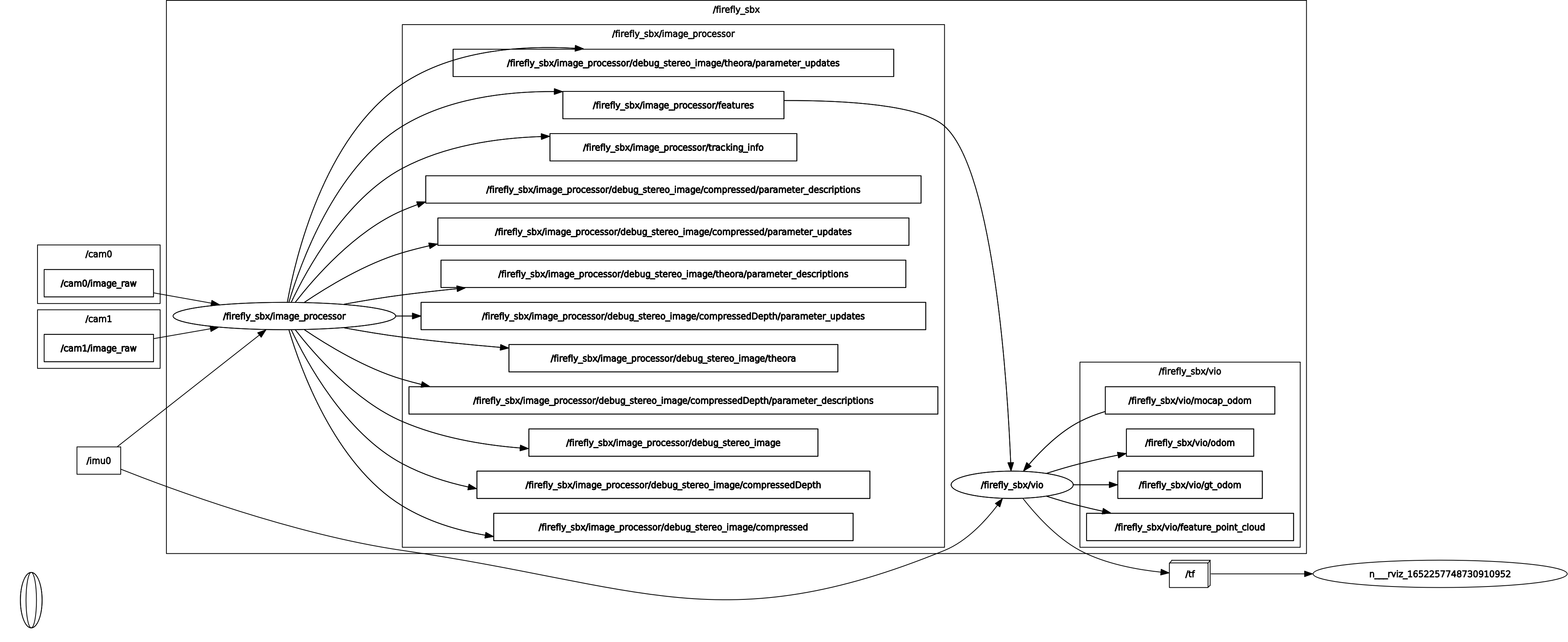
MSCKF的ros graph
视频结果
2 符号表示
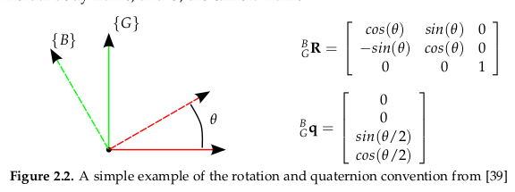
G : 世界坐标系
C : 相机坐标系
B : 机体坐标系
3 概率状态估计
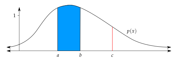
概率论基础
\(P(x = X)\) 在某个范围内的概率等于 概率密度函数 \(p(x)\) 在该范围内的积分
均值和方差
\(\mathbb{E}(x) = \int x p(x) dx\)
\(Var(x) = \mathbb{E}[x - \mathbb{E}(x)^2] = \sigma^2\)
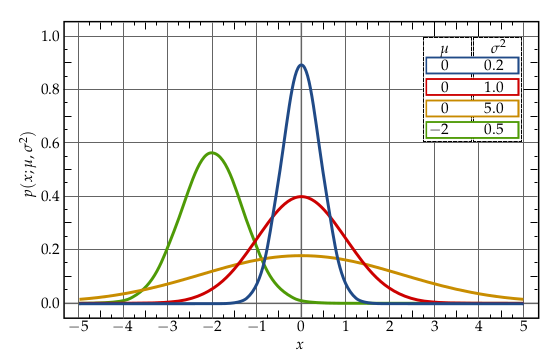
高斯分布
一维高斯密度函数
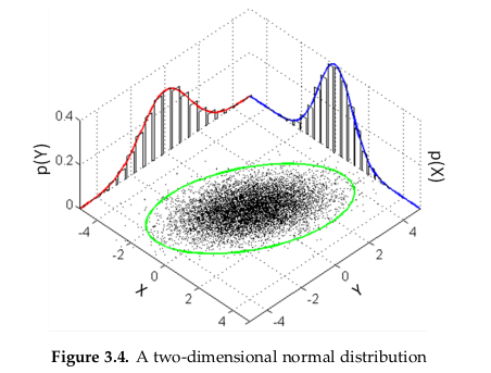
\(N\) 维高斯密度函数
其中:
\[\begin{split}\begin{aligned} Cov(\mathbf{x}, \mathbf{y}) &= \mathbb{E[(\mathbf{x} - \mathbb{E(x)})(\mathbf{y} - \mathbb{E(y)})]} \\ Cov\left(\begin{bmatrix} x_1 \\ x_2 \\ \vdots \\ x_n \end{bmatrix} \right) &= \begin{bmatrix} \sigma_{x_1}^2 & \rho_{(x_1, x_2)}\sigma_{x_1}\sigma_{x_2} & \dots & \rho_{(x_1, x_n)}\sigma_{x_1}\sigma_{x_n} \\ \rho_{(x_2, x_1)}\sigma_{x_2}\sigma_{x_1} & \sigma_{x_2}^2 & \dots & \rho_{(x_2, x_n)}\sigma_{x_2}\sigma_{x_n} \\ \vdots & \vdots & \ddots & \vdots \\ \rho_{(x_n, x_1)}\sigma_{x_n}\sigma_{x_1} & \rho_{(x_n, x_2)}\sigma_{x_n}\sigma_{x_2} & \dots & \sigma_{x_n}^2 \end{bmatrix} \end{aligned}\end{split}\]
条件高斯
边缘化
条件概率
其中:
\(\mathbf{x} \sim N(\mu_x, \Sigma_{xx})\)
\(y = Ax + b, \quad b \sim N(0, Q)\)
4 卡尔曼滤波
4.1 卡尔曼滤波
初始状态估计
预测
更新
4.2 扩展卡尔曼滤波EKF
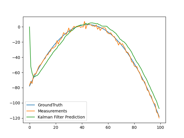
4.3 卡尔曼滤波Python例子
二次函数添加噪点,二次函数
Python例子
import numpy as np

class KalmanFilter(object):
    def __init__(self, F = None, B = None, H = None, Q = None, R = None, P = None, x0 = None):

        if(F is None or H is None):
            raise ValueError("Set proper system dynamics.")

        self.n = F.shape[1]
        self.m = H.shape[1]

        self.F = F
        self.H = H
        self.B = 0 if B is None else B
        self.Q = np.eye(self.n) if Q is None else Q
        self.R = np.eye(self.n) if R is None else R
        self.P = np.eye(self.n) if P is None else P
        self.x = np.zeros((self.n, 1)) if x0 is None else x0

    def predict(self, u = 0):
        self.x = np.dot(self.F, self.x) + np.dot(self.B, u)
        self.P = np.dot(np.dot(self.F, self.P), self.F.T) + self.Q
        return self.x

    def update(self, z):
        y = z - np.dot(self.H, self.x)
        S = self.R + np.dot(self.H, np.dot(self.P, self.H.T))
        K = np.dot(np.dot(self.P, self.H.T), np.linalg.inv(S))
        self.x = self.x + np.dot(K, y)
        I = np.eye(self.n)
        self.P = np.dot(np.dot(I - np.dot(K, self.H), self.P),
          (I - np.dot(K, self.H)).T) + np.dot(np.dot(K, self.R), K.T)

def example():
  dt = 1.0/60
  F = np.array([[1, dt, 0], [0, 1, dt], [0, 0, 1]])
  H = np.array([1, 0, 0]).reshape(1, 3)
  Q = np.array([[0.05, 0.05, 0.0], [0.05, 0.05, 0.0], [0.0, 0.0, 0.0]])
  R = np.array([0.5]).reshape(1, 1)

  x = np.linspace(-10, 10, 100)
  ground_truths = -x**2 - 2*x + 2
  measurements = -(x**2 + 2*x - 2) + np.random.normal(0, 2, 100)

  kf = KalmanFilter(F = F, H = H, Q = Q, R = R)
  predictions = []

  for z in measurements:
    predictions.append(np.dot(H,  kf.predict())[0])
    kf.update(z)

  import matplotlib.pyplot as plt
  plt.plot(range(len(ground_truths)), ground_truths, label = 'GroundTruth')
  plt.plot(range(len(measurements)), measurements, label = 'Measurements')
  plt.plot(range(len(predictions)), np.array(predictions), label = 'Kalman Filter Prediction')
  plt.legend()
  plt.show()

if __name__ == '__main__':
    example()
kalman filter结果
5 IMU
5.1 Accelerometers(加速计)
其中:
\(\mathbf{T}_a\) : 加速度计测量中导致未对准和比例误差的矩阵系数
\(^G\mathbf{a}\) : 全局坐标系中 IMU 的真实加速度,{ B } 表示惯性体(IMU)坐标系。
\(^G\mathbf{g}: \quad \mathbf{g} = (0, 0, -1)^T\)
\(\mathbf{n}_a \sim N(0, N_a)\)
\(\mathbf{b}_a:\) 随时间变化,建模为随机游走过程噪声 \(n_{wa} \sim N(0,N_{wa} )\)
5.2 Gyroscope(陀螺仪)
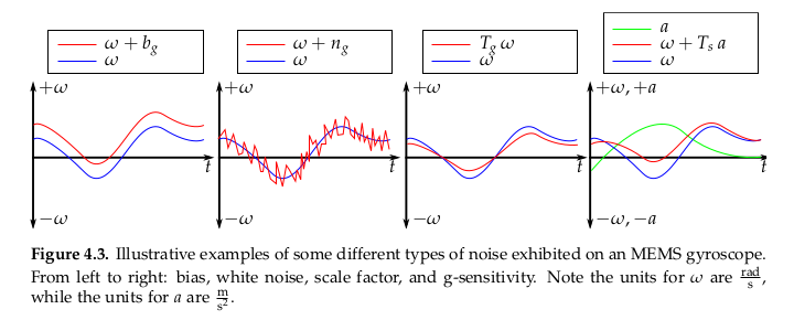
其中:
\(\mathbf{n}_g \sim N(0, N_g)\)
\(\mathbf{b}_g:\) 随时间变化,建模为随机游走过程噪声 \(n_{wg} \sim N(0,N_{wg})\)
5.3 Noise and Bias Characteristics(噪声和零偏特性)
5.4 运动模型
状态向量:
\(_G^I\mathbf{q}(t)^T\) : 代表惯性系到IMU坐标系的旋转
\(\mathbf{b}_g(t)^T\) : 表示在IMU坐标系中测量值线加速度的biases
\(^G\mathbf{v}_I(t)^T\) : 代表IMU坐标系在惯性系中的速度
\(\mathbf{b}_a(t)^T\) : 表示在IMU坐标系中测量值角速度的biases
\(^G\mathbf{p}_I(t)^T\) : 代表IMU坐标系在惯性系中的位置
\(C^I\mathbf{q}(t)^T\) : 表示相机坐标系和IMU坐标系的相对位置,其中相机坐标系取左相机坐标系。
\(^I{\mathbf{p}(t)_C}^T\) : 表示相机坐标系和IMU坐标系的相对位置,其中相机坐标系取左相机坐标系。
\(\mathbf{w}(t)^T = [w_x(t), w_y(t), w_z(t)]^T\) : 是IMU角速度在IMU系中的坐标
IMU的观测值为
将地球自转的影响忽略不计
其中 \(w_{G}\) 为地球的自转速度在 \(G\) 系的坐标
矩阵形式
5.5 状态转移矩阵
性质:
\(\mathbf{\Phi}(t_k, t_k) = \mathbf{I}_{15 \times 15}\)
\(\mathbf{\Phi} \approx I + F \Delta {t}\)
因此:
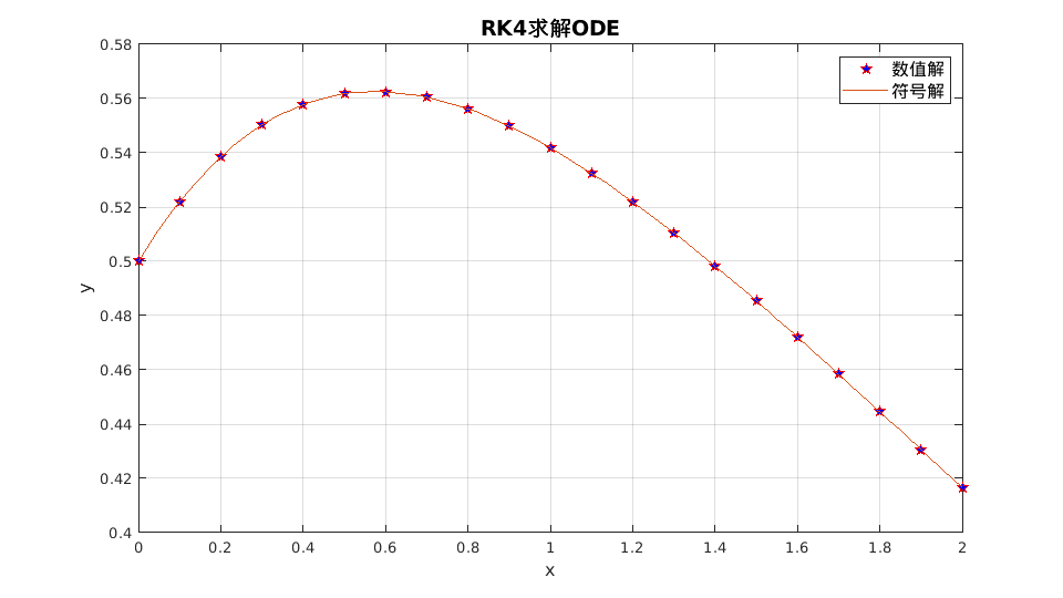
5.6 四阶Runge-Kutta积分
ODE方程:
so that:
例
% 输入参数
fun = @(x, y) (exp(-x) - y) / 2;
x = 0 : 0.1 : 2;
y0 = 1/2;
% 调用RK4函数求解
y = RK4(fun, x, y0);
% 设置图幅
fig = gcf;
fig.Color = 'w';
fig.Position = [250, 250, 960, 540];
% 绘制数值解
p = plot(x, y);
p.LineStyle = 'none';
p.Marker = 'p';
p.MarkerEdgeColor = 'r';
p.MarkerFaceColor = 'b';
p.MarkerSize = 8;
hold on, grid on
% 求解符号解
syms y(x)
equ = 2 * diff(y, x) == exp(-x) - y;
cond = y(0) == 1/2;
y = dsolve(equ, cond);
% 绘制符号解
fplot(y, [0, 2])
% 设置信息
xlabel('x', 'fontsize', 12);
ylabel('y', 'fontsize', 12);
title('RK4求解ODE', 'fontsize', 14);
legend({'数值解', '符号解'}, 'fontsize', 12);
RK4函数如下
function y = RK4(fun, x, y0)

  %RK4 使用经典的RK4方法求解一阶常微分方程。
  % fun是匿名函数。
  % x是迭代区间
  % y0迭代初始值。

  y = 0 * x;
  y(1) = y0;
  h = x(2) - x(1);
  n = length(x);

  for m = 1 : n-1
      k1 = fun(x(m), y(m));
      k2 = fun(x(m)+h/2, y(m)+h*k1/2);
      k3 = fun(x(m)+h/2, y(m)+h*k2/2);
      k4 = fun(x(m)+h, y(m)+h*k3);
      y(m+1) = y(m) + h*(k1 + 2*k2 + 2*k3 + k4) / 6;
  end
end
求解如下:
6 计算机视觉
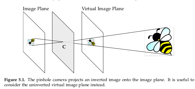
6.1 Pinhole Camera Model(针孔模型)
6.2 相机投影
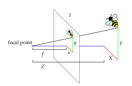
投影变换
6.3 图像畸变
6.4 Triangulation(三角化)
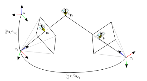
\(C_0\) 帧是第一次观察到该点的相机帧,该点在第 \(i\) 个相机 \(C_i\) 帧中的位置如下。
这可以用逆深度参数化重写,以提高数值稳定性并帮助避免局部最小值
其中:
\(\alpha = \frac{^{C_0}X}{^{C_0}Z}\)
\(\beta = \frac{^{C_0}Y}{^{C_0}Z}$\)
\(\rho = \frac{1}{^{C_0}Z}\)
6.5 高斯牛顿最小化
损失函数cosnt function
雅可比矩阵Jacobian
其中:
参数更新
6.6 Feature Points Detect
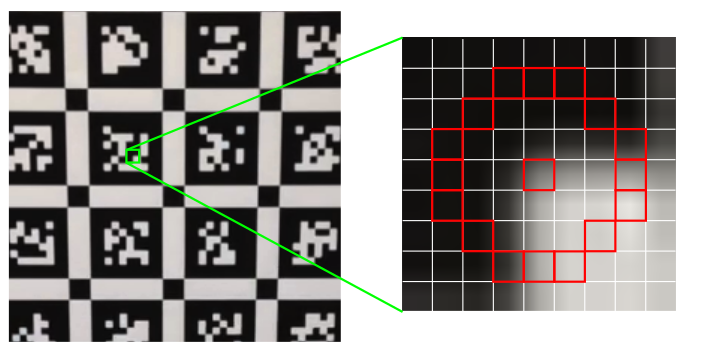
6.7 Feature Matching
7 MSCKF-VIO
EuRoC数据集
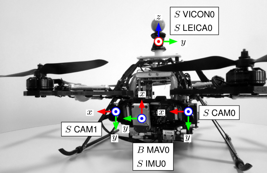
微型飞行器(MAV)上收集的视觉惯性数据集
使用的机型为:Asctec Firefly六角旋翼直升机
觉惯性测量的传感器包括:视觉(双相机)惯性测量单元(IMU)
视觉惯性传感器与groundtruth数据之间,通过外部校准使得时间戳同步。
groundtruth采集
Leica MS50 激光跟踪扫描仪:毫米精确定位
Note
LEICA0:激光追踪器配套的传感器棱镜【prism】
Leica Nova MS50: 激光追踪器,测量棱镜prism的位置,毫米精度,帧率20Hz,
数据集内包含的数据
Vicon 6D运动捕捉系统
Note
VICON0:维肯动作捕捉系统的配套反射标志,叫做marker
Vicon motion capture system: 维肯动作捕捉系统,提供在单一坐标系下的6D位姿测量,测量方式是通过在MAV上贴上一组反射标志,帧率100Hz,毫米精度
视觉惯性传感器:
Note
双相机 (Aptina MT9V034型号 全局快门, 单色, 相机频率20Hz)
MEMS IMU (ADIS16448型号 , 测量角速度与加速度,测量频率200 Hz)(以视觉图像的时间戳为基准进行对齐)
groundtruth
Note
Vicon运动捕捉系统【marker】(6D姿势)
Leica MS50激光跟踪仪(3D位置)
Leica MS50 3D 结构扫描
传感器校准
Note
相机内参
相机-IMU外参
文件名 MH_01_easy [工厂场景]
Note
- ——mav0
- — cam0
data :图像文件 data.csv :图像时间戳 sensor.yaml : 相机参数【内参fu,fv,cu,cv、外参T_BS(相机相对于b系的位姿)、畸变系数】
- — cam1
data :图像文件 data.csv :图像时间戳 sensor.yaml : 相机参数【内参fu,fv,cu,cv、外参T_BS(相机相对于b系的位姿)、畸变系数】
- — imu0
data.csv : imu测量数据【时间戳、角速度xyz、加速度xyz】 sensor.yaml : imu参数【外参T_BS、惯性传感器噪声模型以及噪声参数】
- — leica0
data.csv : leica测量数据【时间戳、prism的3D位置】 sensor.yaml : imu参数【外参T_BS】
- — state_groundtruth_estimae0**
data.csv :地面真实数据【时间戳、3D位置、姿态四元数、速度、ba、bg】 sensor.yaml :
在每个传感器文件夹里配一个senor.yaml文件,记录传感器相对于Body坐标系的坐标变换,以及传感器自身参数信息
groundtruth输出格式
timestamp,
p_RS_R_x [m]
p_RS_R_y [m]
p_RS_R_z [m]
q_RS_w []
q_RS_x []
q_RS_y []
q_RS_z []
v_RS_R_x [ m/s]
v_RS_R_y [ m/s]
v_RS_R_z [ m/s]
b_w_RS_S_x [rad /s]
b_w_RS_S_x [rad /s]
b_w_RS_S_z [rad /s]
b_a_RS_S_x [rad /s]
b_a_RS_S_y [rad /s]
b_a_RS_S_z [rad /s]
timestamp:18位的时间戳
position:MAV的空间3D坐标
p_RS_R_x [m]
p_RS_R_y [m]
p_RS_R_z [m]
传感器安装的相对位置
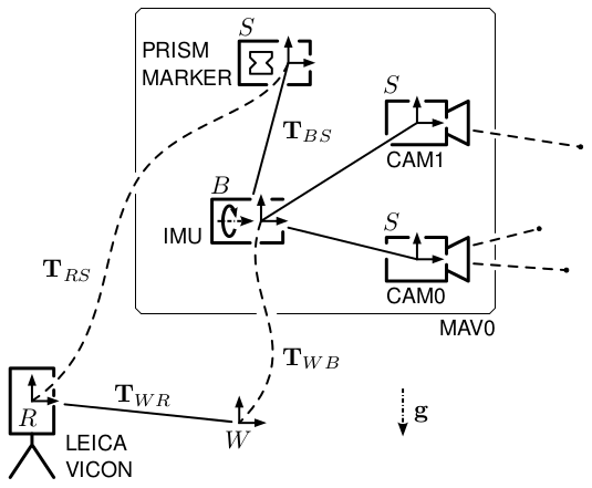
机体上载有4个传感器,其中prism和marker公用一个坐标系 无人机的body系 以IMU传感器为基准,即,imu系为body系。
EuRoC数据集的使用
EuRoC数据集可用于视觉算法、视觉惯性算法的仿真测试
在VIO算法中涉及到很多坐标系的转换、在精度测量过程中也需要进行统一坐标系
Note
- 传感器数据的读取
以相机图像与imu测量作为算法输入,首先就是要进行数据读取、将输入输出模块化
- 建立统一坐标系
传感器放置于统一平台上,但每个传感器都有其各自的坐标系,索性EuRoC中给出了所有传感器相对于机体body系的相对位移(sensor.yaml文件中的T_BS),因此可以将各传感器的位姿数据统一到统一坐标系下,但实际使用中需要根据代码情况灵活运用。
- 坐标系变换:
下标表示形式【 矩阵坐标系之间的变换矩阵的下标采用双字母进行标注】 如:旋转矩阵R_BC,表示从c系旋转到b系的变换阵
7.1 Overview
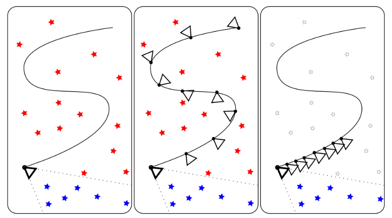
传统的EKF-SLAM框架中,特征点的信息会加入到特征向量和协方差矩阵里,这种方法的缺点是特征点的信息会给一个初始深度和初始协方差, 如果不正确的话,极容易导致后面不收敛,出现inconsistent的情况。MSCKF维护一个pose的FIFO,按照时间顺序排列, 可以称为滑动窗口,一个特征点在滑动窗口的几个位姿都被观察到的话,就会在这几个位姿间建立约束,从而进行KF的更新。 如下图所示, 左边代表的是传统EKF SLAM, 红色五角星是old feature,这个也是保存在状态向量中的,另外状态向量中只保存最新的相机姿态; 中间这张可以表示的是keyframe-based SLAM, 它会保存稀疏的关键帧和它们之间相关联的地图点; 最右边这张则可以代表MSCKF的一个基本结构, MSCKF中老的地图点和滑窗之外的相机姿态是被丢弃的, 它只存了滑窗内部的相机姿态和它们共享的地图点.
7.2 前端
跟踪流程
初始化Initialization

trackFeatures

twoPointRansac
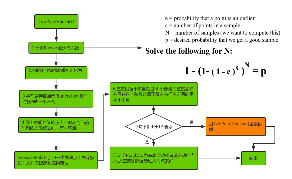
对极几何可约束
\(p_1 = [x_1, y_1, 1]^T\)
\(p_2 = [x_2, y_2, 1]^T\)
展开之后我们可以得到
7.3 State Representation

publish
uint64 id
# Normalized feature coordinates (with identity intrinsic matrix)
float64 u0 # horizontal coordinate in cam0
float64 v0 # vertical coordinate in cam0
float64 u1 # horizontal coordinate in cam0
float64 v1 # vertical coordinate in cam0
其实前端基本上可以说是非常简单了,也没有太多的trick,最后我们来看一下前端的跟踪效果的动图:
7.4 Propagation
误差状态协方差更新
IMU误差状态方程离散化:
从 \(t_{k}\) 到 \(t_{k+1}\) 的状态转移矩阵 \(\Phi_{k}\) 和噪声项 \(Q_{k}\) 为:
其中:
\(Q = \mathbf{n_I n_I^{T}}\)
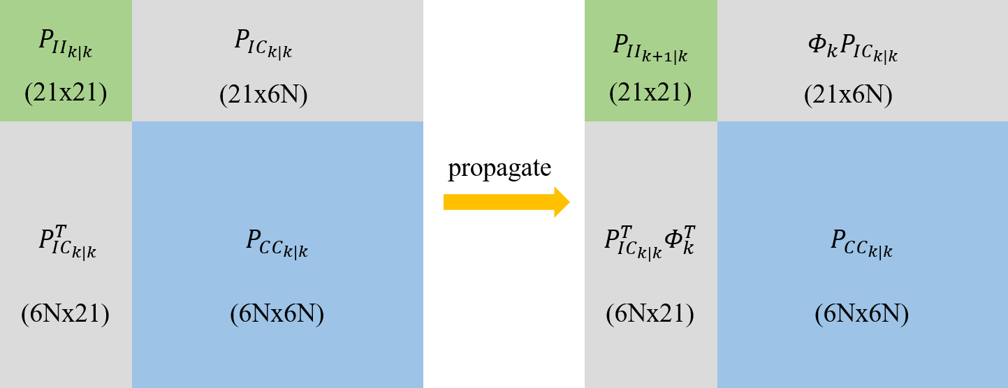
\(k\) 时刻 \(\mathbf{X}_{IMU}\) 变化对系统误差状态协方差矩阵 \(P_{k|k}\) , 系统误差状态协方差矩阵为:
\(k+1\) 时刻预测的IMU误差状态协方差矩阵为
\(k+1\) 时刻预测的系统误差状态协方差矩阵为:
整个状态(IMU+Camera)的covariance传播过程如图所示:
7.5 Augmentation
MSCKF系统的误差状态向量
它包括 \(IMU\) 误差状态与 \(N\) 个相机状态。在没有图像进来时,对 \(IMU\) 状态进行预测, 并计算系统误差状态协方差矩阵;在有图像进来时,根据相机与 \(IMU\) 的相对外参计算当前相机的位姿。 然后将最新的相机状态加入到系统状态向量中去,然后扩增误差状态协方差矩阵。
状态向量扩增
根据预测的IMU位姿和相机与IMU的相对外参计算当前相机位姿:
然后将当前相机状态 \(_G^{C}\hat{q}, ^{G} \hat{p}_{C}\) 加入到状态向量。
\(_G^{C}\hat{q}\) : 相机的方向
\(^{G} \hat{p}_{C}\): 相机的位置
误差状态协方差矩阵扩增
系统新误差状态 \(X_{new}\) 与系统原误差状态 \(X_{old}\) 的关系为:
其中
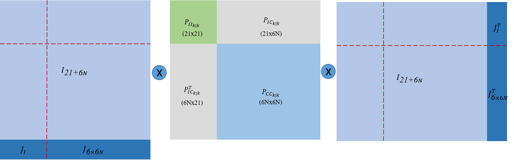
\(J\) 是新增相机误差状态对原系统误差状态的Jacobian:
假设上一时刻共有N个相机姿态在状态向量中,那么当新一帧图像到来时,这个时候整个滤波器的状态变成了 \(21 + 6(N+1)\) 的向量, 那么它对应的covariance维度为 \((21 + 6(N+1)) \times (21 + 6(N+1))\) 。求出 \(J\) 后,误差状态协方差矩阵扩增为:
这个过程对应如下图过程:
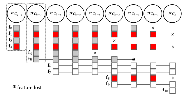
7.6 Update Step
MSCKF的观测模型是以特征点为分组的,我们可以知道一个特征(之前一直处于跟踪成功状态)会拥有多个Camera State. 所有这些对于同一个3D点的Camera State都会去约束观测模型. 那这样其实隐式的将特征点位置从状态向量中移除, 取而代之的便是Camera State. 我们考虑单个feture \(f_j\) ,假设它所对应到 \(M_j\) 个相机姿态 \([{}_G^{C_{i}}\mathbf{q}, {}^G \mathbf{p}_{C_i}]^T, i \in j\) 。 当然双目版本的包含左目和右目两个相机姿态, \([{}_G^{C_{i,1}}\mathbf{q}, {}^G \mathbf{p}_{C_i, 1}]^T\) 和 \([{}_G^{C_{i,2}}\mathbf{q}, {}^G \mathbf{p}_{C_i, 2}]^T\) 右相机很容易能通过外参得到. 其中双目的观测值可以表示如下:
而特征点在两个相机坐标系下可以分别表示为:
其中 \({}^{G}\mathbf{p}_j\) 是特征点在惯性系下的坐标,这个是通过这个特征点的对应的所有camera state三角化得到的结果. 将观测模型在当前状态线性化可以得到如下式子:
其中 \(\mathbf{n}^{j}_{i}\) 是观测噪声, \(\mathbf{H}_{C_{i}}^{j}\) 和 \(\mathbf{H}^{f_j w}\) 是对应的雅克比矩阵。 对应到的是单个特征点对应的其中某一个相机姿态, 但是这个特征点会对应到很多相机姿态。
但是这个其实并不是一个标准的EKF观测模型,因为我们知道 \(\mathbf{\tilde{p}_j}\) 并不在我们的状态向量里边, 所以做法是将式子中红色部分投影到零空间, 假设 \(\mathbf{H^{f_{j}w}}\) 的left null space为 \(\mathbf{V}^T\) , 即有 \(\mathbf{V}^T \mathbf{H^{f_{j}w}} = 0\), 所以:
这样就是一个标准的EKF观测模型了,下面简单分析一下维度.分析时针对单个特征点, 我们知道 \(\mathbf{H^{f_{j}w}}\) 的维度是 \({4M_j} \times 3\) , 那么它的left null space的维度即 \(\mathbf{V}^T$的维度为$(4M_j -3) \times 4M_j\) , 则最终 \(\mathbf{H}^{j}_{0} \mathbf{x}\) 的维度变为 \((4M_j-3) \times 6\) , 残差的维度变为 \((4M_j-3) \times 1\) , 假设一共有L个特征的话,那最终残差的维度会是 \(L (4M_j-3) \times 6\).
7.7 Post EKF Update
大致是有两种更新策略,假设新进来一帧图像,这个时候会丢失一些特征点,这个时候丢失的特征点(且三角化成功)用于滤波器更新,如下图所示: